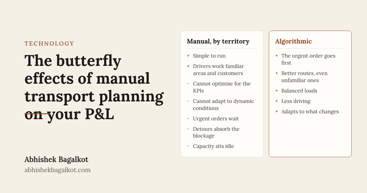
The butterfly effects of manual transport planning on your P&L
Operating a vehicle fleet for delivery or collection of goods to & from various locations is a very common industry use case. Every day, the dairy industry delivers fresh milk from millions of cattle farmers to billions of consumers on time. Large FMCGs refill their inventory across millions of retail stores, e-commerce delivers customer orders and municipal bodies evacuate garbage. Companies depend on the efficient functioning of vehicle fleets to deliver high quality, fresh products on time and keep customer promises.
These fleets are purchased or engaged in advance. Drivers assemble at depots at the beginning of a shift. Routes are then assigned to drivers to complete multiple finite sets of tasks, the status of which is often tracked digitally.
We are able to see such vehicle operations in our everyday lives. But the science of assigning vehicles and routes, called transport planning, is not well understood by most of us. Not only by the general public, but even so by some experienced transport managers. Optimised transport planning is often a counter-intuitive process with many moving variables.
Yet, there is much to be gained from studying & improving our transport planning. Delivering customer orders on time, every time increases customer delight and repeat orders. Delivering perishable goods on time is so critical, failing which a double whammy would hit the P&L’s top line and the bottom line alike. Ensuring product availability after a successful marketing campaign can really accelerate revenue.
This article explains the benefits of an algorithmic transport planning approach for vehicle and route assignment. This approach can be used by planners to optimise transport operations for KPI improvement or to rapidly respond to changing realities or obstacles in the transport operations.
Manual planning methods
Traditionally, transport planning most often defaults to dividing the service areas into smaller territories first. A large service area is divided into smaller non-intersecting territories, that can be serviced by a single or small collection of vehicles. Post which vehicle assignment and route planning is done.
The division of a large service area into sub territories makes the problem easier for human conceptualisation. A collection of manageably smaller graphs with limited number of continuous vertices traversed by single vehicle is easier to conceptualise and solve for. It divides a large problem into several smaller ones, that do not interact with each other.
Yet, business KPIs like total fuel cost, average turnaround time, total driver hours etc. not only aggregate together, but also interact with one another in complex ways. One local optimisation, like choosing the shortest route for that day’s order, may adversely affect a global aggregate KPI of uniform capacity utilisation.
Manual transport planning cannot account for such higher order interactions between competing objectives or take into account that locally optimised KPIs may not aggregate well at a global business level.
Fundamentally, manual transport planning has the following features
1. Cannot optimise for the KPIs
Territories are drawn around geography, not around cost per drop, on-time delivery, or fleet utilisation. Each vehicle is planned within its own territory, so the fleet is never optimised as a whole.
2. Cannot adapt to dynamic conditions
Manual planning is time-consuming. Redoing the plan when ground reality changes is highly time-consuming. If a driver is absent or a vehicle breaks down, the situation often results in unacceptable delays. Yet, road conditions, traffic conditions and delivery urgencies change every day.
How territory-based planning works
Territory planning divides the whole service area into smaller chunks serviced by an individual vehicle. The diagram below demonstrates this.
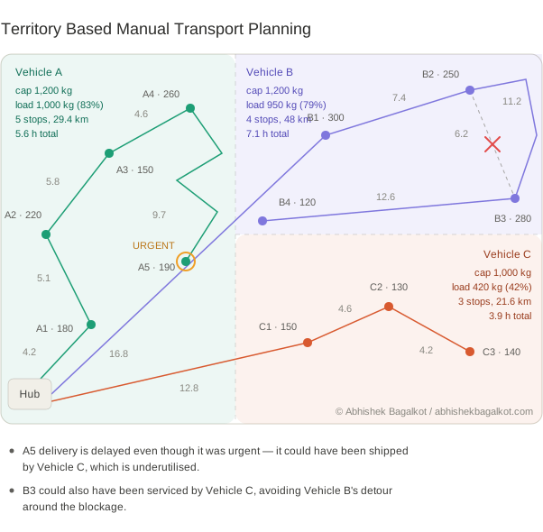
The planner assigns each delivery to the vehicle that owns its territory. The driver then sequences the stops, usually by habit. The map shows three consequences:
- Urgent orders wait. A5 is urgent but sits at the end of Vehicle A’s route, so it’s delivered last. Vehicle C, which is closer and has room, never gets it.
- Detours absorb the blockage. When Vehicle B’s usual road is blocked, it drives 11.2 km around it, even though a 6.2 km alternative existed.
- Capacity sits idle. Vehicle C runs at 42% while A and B are near full.
None of these show up as planning errors. They show up as overtime, fuel bills, and missed deliveries.
How algorithmic transport planning works
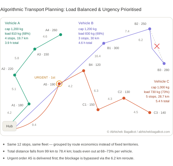
With the same stops and the same fleet, the algorithm drops the territories. It considers all deliveries, vehicle capacities, travel distances, and priorities together, then recommends the routes. The result:
- The urgent order goes first. A5 moves to Vehicle C and becomes its first stop.
- Better routes, even unfamiliar ones. Vehicle B takes the shorter reroute around the blockage because of the algorithmic route recommendation.
- Balanced loads. Utilisation evens out at 68–73% across all three vehicles.
- Less driving. Total distance falls from 99 km to 78.4 km, about 21% less. The longest working day drops from 7.1 to 5.4 hours.
Because the plan is recalculated each time, it adapts to what changes: new orders, blockages, and shifting priorities.